Introduction

Every morning Monday to Friday, A frenzy is created mostly through various social networking groups and partly by pre-opening shows on business channels to impress upon potential investor about likely move in major Indian indexes/stocks by analyzing behavior of other global indexes to profit in very short term. The discourse opens scope for another analysis to understand the relation if any between Indian and other global indexes.

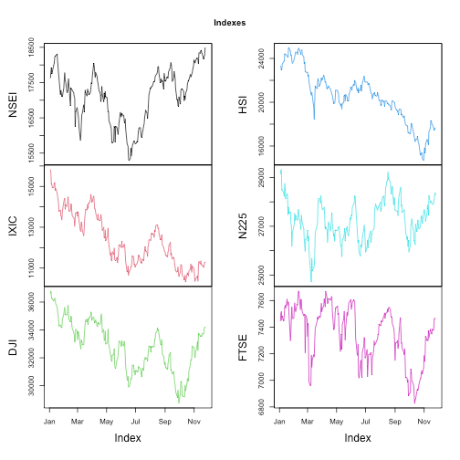
Initial Plot

This is how major Indexes performed during the current calendar year. A simple optical observation reveal that in second half of the year Nifty50 and BankNifty outperformed global peers by miles.

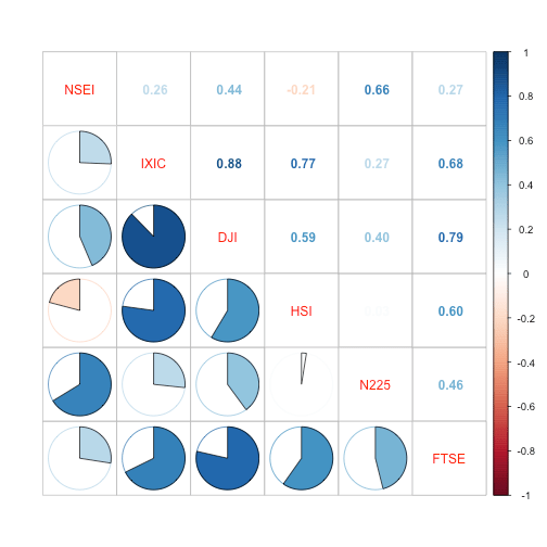
Static correlation

A static correlation based on daily data. This shows that correlation is negative with Hangseng, poor with US Index and comparably strong with Nikkai.

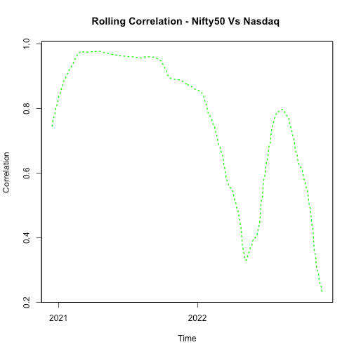
Rolling Correlation

Static correlation does not provide any direction. Hence, rolling correlation is calculated to observe the movement over the period.
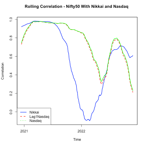
Outcome is quite informative, correlation used to be very high b/w NIFTY50 and NASDAQ, however it started dropping around later half of previous year and is currently hovering near the the lowest level.

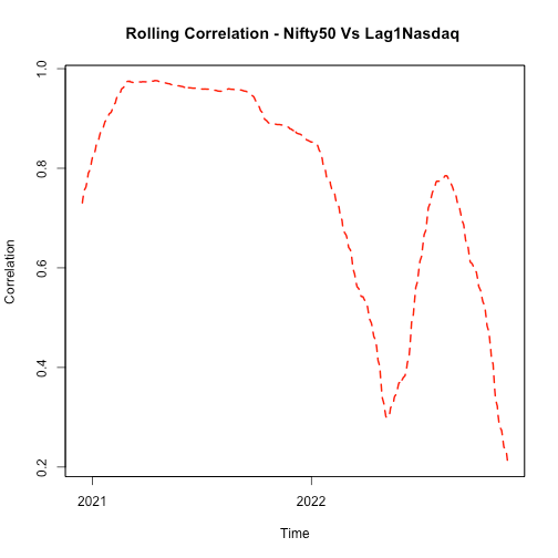
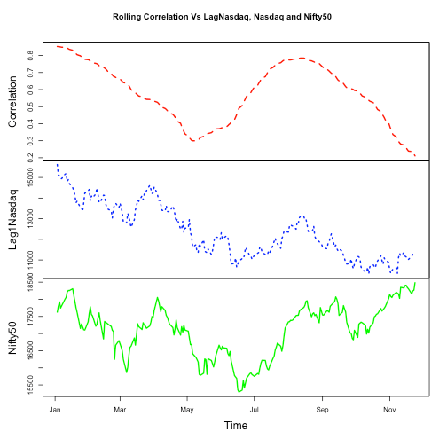
Correlation is also calculated b/w lag1 NASDAQ and NIFTY50 since US is behind one day. As expected, results are not very different.

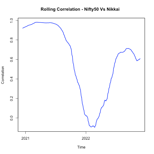
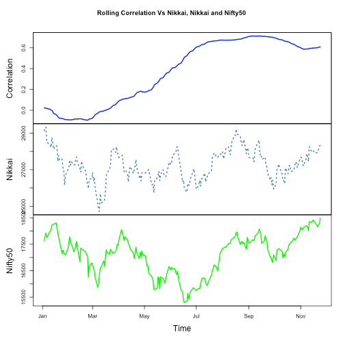
Correlation B/w NIFTY50 and Nikkai. It is interesting to note that correlation started declining in later part of previous year and rising again.

Few charts to observe the movements.

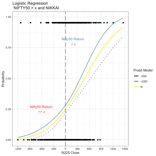
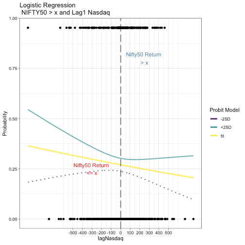
Logistic Regression

Although it is quite clear that in a very short period, at least US index movement does not mean a lot. However, carry out a logistic regresion for NASDAQ and Nikkai, results are displayed by way of chart appended below.

## 
## Call:
## glm(formula = I(df1[, n1] > 100) ~ df1[, n2], family = binomial(link = "probit"), 
##     data = df1)
## 
## Deviance Residuals: 
##     Min       1Q   Median       3Q      Max  
## -1.5781  -0.7950  -0.6284   1.0554   2.9975  
## 
## Coefficients:
##               Estimate Std. Error z value Pr(>|z|)    
## (Intercept) -0.6806971  0.0521966 -13.041  < 2e-16 ***
## df1[, n2]    0.0014205  0.0001757   8.087 6.14e-16 ***
## ---
## Signif. codes:  0 '***' 0.001 '**' 0.01 '*' 0.05 '.' 0.1 ' ' 1
## 
## (Dispersion parameter for binomial family taken to be 1)
## 
##     Null deviance: 881.65  on 755  degrees of freedom
## Residual deviance: 805.22  on 754  degrees of freedom
## AIC: 809.22
## 
## Number of Fisher Scoring iterations: 4

## 
## Call:
## glm(formula = I(df1[, n1] > 100) ~ df1[, n3], family = binomial(link = "probit"), 
##     data = df1)
## 
## Deviance Residuals: 
##     Min       1Q   Median       3Q      Max  
## -0.9143  -0.7997  -0.7779   1.5490   1.7147  
## 
## Coefficients:
##               Estimate Std. Error z value Pr(>|z|)    
## (Intercept) -0.6133662  0.0488719 -12.550   <2e-16 ***
## df1[, n3]   -0.0002736  0.0002435  -1.124    0.261    
## ---
## Signif. codes:  0 '***' 0.001 '**' 0.01 '*' 0.05 '.' 0.1 ' ' 1
## 
## (Dispersion parameter for binomial family taken to be 1)
## 
##     Null deviance: 881.65  on 755  degrees of freedom
## Residual deviance: 880.38  on 754  degrees of freedom
## AIC: 884.38
## 
## Number of Fisher Scoring iterations: 4

Summary

Contrary to general understanding, Nifty50 shares the best correlation
with Nikkai not the US Index in the current context. Bettter look east than West!

---